OSRS Grand Exchange Price Predictions

Stock price predictors have been a heavily researched topic in the intersection of machine learning, data science, and finance. The guaranteed profits of being able to predict the stock market are immense, so why hasn’t it been done?

The problem lies within the very data itself. Stock data is abundant, some datasets contain the very beginning of the stock market from 200 years ago. However, this data is extremely noisy, there are simply too many factors that play into the price of stocks, such as embargos, politics, recessions, and public perception - all of which is not included in the data. Some believe that it is all noise, this is called the Random Walk Hypothesis. The Random Walk Hypothesis suggests that there are no coherent patterns in stock data, and that it is all random. Can we test this hypothesis in a virtual economy?

The OSRS Grand Exchange

OSRS (Old School Runescape) is a popular MMORPG with a free market called the Grand Exchange where players can sell their items. The Grand Exchange mirrors real-world economic principles, such as inflation, making it an ideal platform for predictive models.

To collect data for this project I used an API called weirdgloop which contains 15 years of historical data of item prices.

The Model

There are multiple time series models to choose from, however, I will be using an LSTM for its balance between accuracy and simplicity. Random forest regressors are simple and are computationally cheap, but may lack accuracy. Whereas a transformer, although being on the cutting edge of machine learning, is complex and computationally expensive.

Brief Explanation of LSTMs

An LSTM (Long Short-Term Memory) is a neural network that specializes in time-series data. It does this by having a feedback loop in each node of the network. RNNs do exactly this but are unable to effectively take in more data as the length of recurrent data increases, due to constraints in memory as well as the exploding/vanishing gradient problem.

An LSTM mitigates this issue by applying a gate mechanism, by using a number of transformations and weights the LSTM is able to dictate which data to commit to its “long term memory” and which data to “forget”.

The Challenges of Time Series Forecasting

Stock data is highly volatile, with high fluctuations in data due to outer influences which are not apparent in previous time steps. This noise serves as a mask, hiding any apparent structure in the data, if there is any at all. This can severely hinder our LSTM’s ability to draw from these patterns to make effective predictions, as such, caution will be taken ahead to mitigate the effects of overfitting as much as possible.

Another challenge apparent in stock data is its non-stationarity. Non-stationarity describes the datasets tendency to have changing properties such as variance and covariance overtime. For example, stock data has a tendency to constantly increase in price due to economic factors such as inflation. This can further obscure underlying trends that can be used to forecast future prices.

Often, time series forecasting models are trained without addressing these issues. As a result the model heavily overfits by predicting prices from the day before, essentially saying that the only underlying pattern found is that the price of an item in the future is similar to the price of the previous day. This results in a neural network with low error, and results that look nearly identical to the ground truth, but with a time lag. This is often misrepresented as a good result when in reality the model is useless.

Addressing the Issues of Time Series Forecasting

These issues are severe and will hinder the accuracy of the model if left unaddressed. In some circumstances, such as real stock data, these issues cannot reliably be addressed due to severe noise.

Firstly, let's start by addressing issues in the data itself. The easiest of which being the non-stationarity of the data. To resolve this we will transform the data by taking the derivative, or the percent change, of the data. We will then use previous changes in price to predict future changes in price, as opposed to the previous method of using current price to predict current price. Although this seems to reframe the problem, in a practical sense, it allows us to know when to sell or buy an item, which is the main objective.

To address the volatility of the data, an exponential moving average is applied to remove short term fluctuations and uncover underlying trends. The moving average must be used sparingly, as a heavy moving average can cause a delay due to it averaging multiple previous data points with the current data point.

Addresssing Overfitting in LSTMs

LSTMs are complex models with gating mechanisms designed to capture long term dependencies. As such LSTMs are prone to overfitting on noise and sequences, and requires more data to train.

Data Cleaning

Using the previous methods the dataset is as clean as we can get it, but it is not perfect. Many of the choices in your model architecture and training parameters have a large impact on overfitting.

Model Complexity

Model complexity can have a large impact on the ability to generalize data. A more complex model is more likely to fit on smaller, possibly noisier details. For this reason I keep the model size small with a single LSTM block followed by 2 dense blocks, more details on that in the implementation section.

Loss Function

Now, a very important parameter is the loss function. The loss function is a function that transforms the error to help a model learn. Some loss functions like Mean Squared Error (MSE) take the square of error, causing outliers to explode and play a more significant impact on model weights. Whereas functions like mean absolute error (MAE) treat error linearly. By choosing a proper loss function we can prevent the model from overfitting on outliers.

Let’s evaluate the strengths and weaknesses of the previously mentioned loss functions.

Mean Squared Error

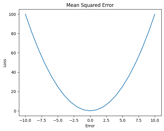
Mean squared error is the most common loss function used in most neural networks. It calculates the square of the error between the predicted and true labels.

Pros:

• Computationally cheap
• Emphasizes large error

Cons:

• Sensitivity to outliers

The sensitivity to outliers plays a large role in this case, since our data is extremely noisy and volatile. Using this means that our network will weigh large fluctuations in data higher than other errors, causing our model to overfit.

Mean Absolute Error

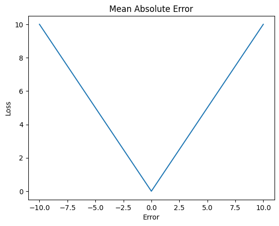
On the opposite end of the spectrum is mean absolute error. MAE takes the magnitude of the error instead of squaring it. This introduces its own strengths in weaknesses.

Pros:

• Less sensitivity to outliers

Cons:

• Less sensitivity to small error
• Slower convergence

As we can see, MAE solves our main issue with MSE, however it introduces its own issues as well. Because it weighs all errors equally, small errors may go unnoticed causing slow convergence and possible biasing. Thankfully, there is a balance to be found.

LogCosh Error

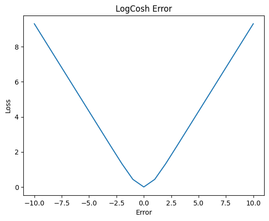
LogCosH, takes the log of the hyperbolic cosine of the error. Lets go step by step, firstly the hyperbolic cosine function is applied to our error. Like MSE this weighs the large error more heavily. The log is then taken to scale these large values down, insuring stability and less sensitivity to outliers.

Pros:

• Less sensitivity to outliers
• Weighs large and small error accordingly
• Allows for proper convergence/li>

Cons:

• More computationally expensive

As you can see, this strikes a balance between MSE and MAE, creating the perfect loss function for our purposes.

Weight Decay

Weight decay, often called L2 regularization, is a regularization technique that helps prevent a model overfitting by penalizing the model complexity. It does this by adding a term that is proportional to the sum of the weights to the loss function. This penalizes large weights that make the model too complex.

Dropout

Dropout is the most common method of overfitting prevention. Dropout works by turning off a specified percentage of random nodes in a layer of a neural network to prevent codependency between nodes. Although simple this is still one of the most effective ways to prevent overfitting.

Early Stopping

Early stopping is a method to prevent overfitting. It does this by monitoring the validation losses and stops training after a specified number of attempts, this number is called the patience. By doing this it effectively finds the optimal number of epochs to train the model for.

Implementation

Using the many data tailoring and regularization techniques above in tandem will help alleviate some of the issues in LSTMs and time series forecasting.To implement these techniques I will be using the Python library Pytorch to design the network and Numpy and Pandas to tailor the data. The code can be found on the Github listed here https://github.com/ShawnPatrick-Barhorst/OSRS_GE_LSTM .

In summary, I modify the existing dataset by taking the percent change between price each day and using an exponential moving average with a small center of mass(COM) of 10.

The LSTM model consists of a single LSTM block with an LSTM layer followed by a batch normalization, a LeakyRelu activation function and a dropout of 30%. The model is then followed by two dense layers each with a batch normalization, a LeakyRelu activation function and a dropout of 30%. This is a very simple neural network architecture that implements the methods above to prevent overfitting.

The custom training loop is also fairly standard, using an Adam optimizer with a learning rate of 0.001 and a weight decay of 0.01. The training loop implements early stopping by comparing the validation score to the previous best validation score with a patience parameter of 5. This means that there are 5 opportunities for the model to decrease the validation loss before the training stops.

The model is then trained using a subset of 100 items, chosen due to memory constraints, with a ratio of 80% training and 20% validation. A sliding window is then used to create an array of 30 data points to be used as input, with the 31st data point being used as the label. This means that using 30 days of previous data we should be able to predict the price of an item 1 day in advance. To predict more than 1 day ahead a method of recursive series forecasting is used to append the predicted sample to the original input and repeat the prediction again. The model is trained for a maximum of 20 epochs but due to early stopping, stops at epoch 14.

Results

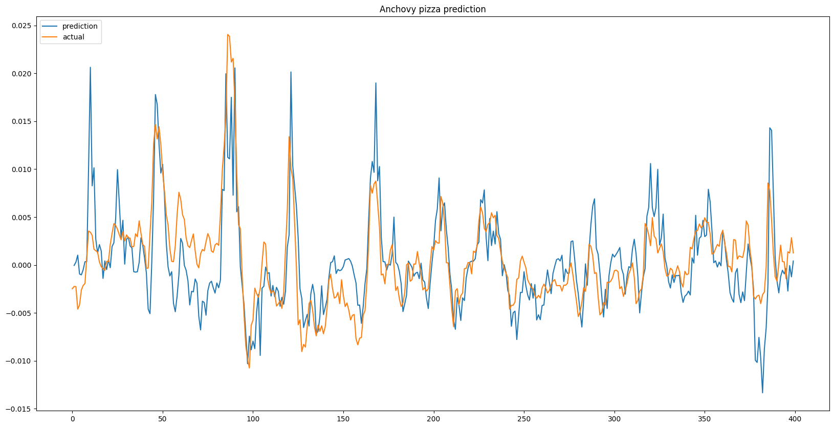
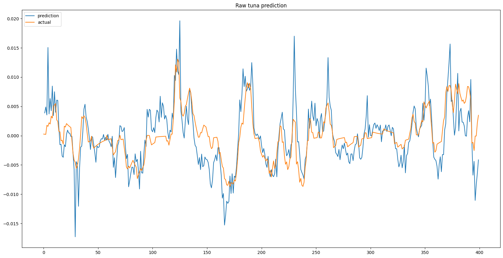
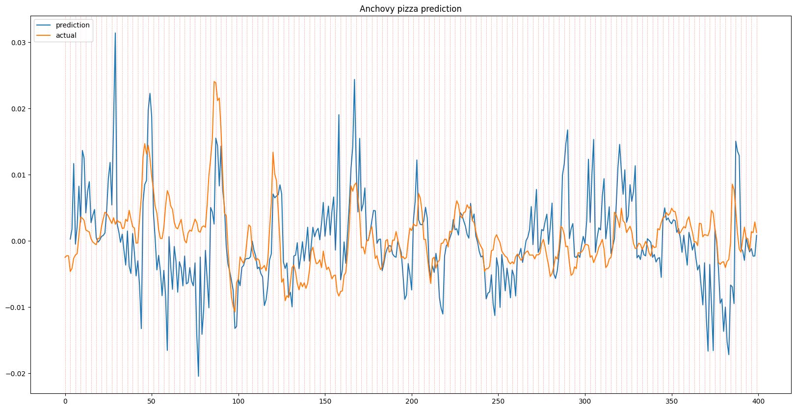
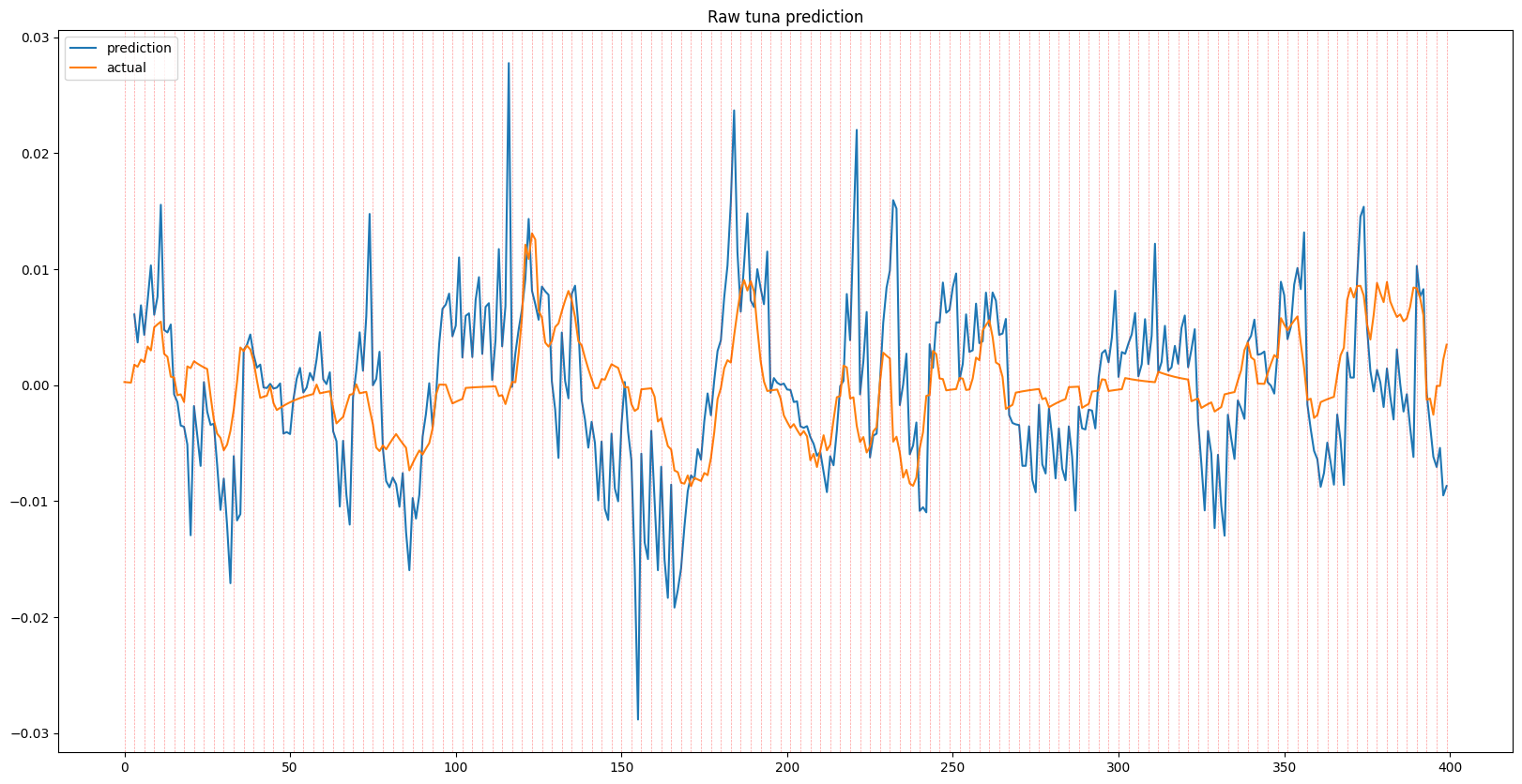
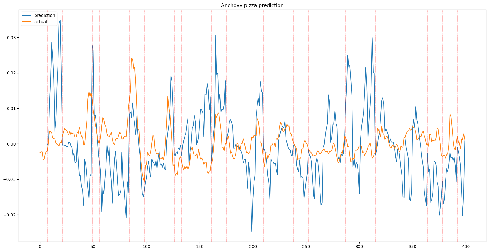
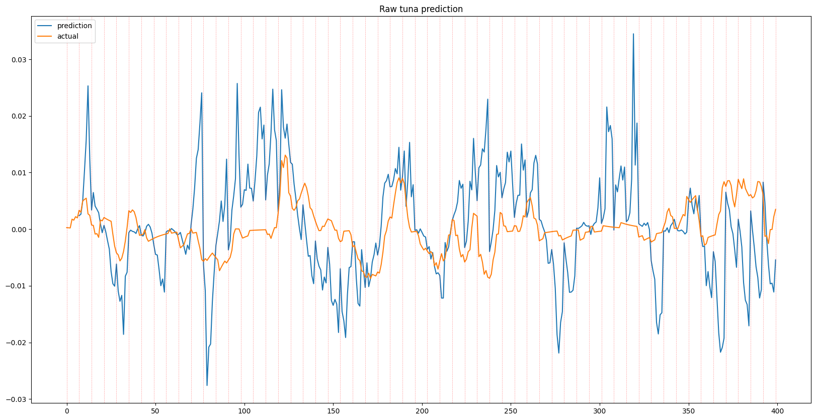
The results shown below displays a series of predictions for each given item, each 1, 3, and 7 days in advance, alongside the ground truth. While some predictions show the effects of time lag due to overfitting, the model general is able to predict trends in item prices. When looking at the recursive outputs in the 3 and 7 day predictions, the predictions do begin to become more erratic due to the error growing as input with error is being fed into the model, however it holds up well and in some instances can successfully predict multiple days in advance.

Single Day Prediction

Recursive 3 Day Prediction

Recursive 7 Day Predictions

Conclusion

The results above show that although noisy, there is a learnable underlying pattern, which means that it isn’t completely noise as suggested by random walk theory, at least for Runescape Grand Exchange data.

Due to the simplicity of the Grand Exchange and Runescapes in-game economy, this doesn’t mean that the same is applicable to real world stock data, which has much more outer influences. However this remains an interesting showcase of the capabilities of LSTMs.

There are a multitude of ways to improve the given results, for example, using an attention mechanism in the LSTM network or using one of the new cutting edge forecasting models such as XLSTM or MAMBA. For the time being, I will leave this project as is, as I move on to other projects.

Thank you for reading.